Chapter 6 Trends of household-level data

In this section, I present the trend of variables in the household level data.

library(tidyverse) 
library(knitr)
library(kableExtra)

list_HH <- list.files(path = "./../exported", pattern = "^HH.*\\Rds$")

HH <- NULL
for (year in list_HH) {
  HH <- assign(year, readRDS(paste0("./../exported/",year))) %>% 
    filter(!is.na(weight)) %>%
    mutate(year = parse_number(year)) %>%
    bind_rows(HH)
  rm(list=year)
}

## Part 1 Tables
HH %>%
  mutate(rural = (urban=="R")*100,
         literate_share = literates/size*100,
         student_share = students/size*100,
         worker_share = employeds/size*100,
         female_head = (gender=="Female")*100,
         age_head = age,
         married_head = (maritalst=="Married")*100 ) %>%
  group_by(year) %>%
  summarize(across(c(khanevartype, rural, size, literate_share, student_share, worker_share, female_head, age_head, married_head),
                   ~weighted.mean(.x,weight,na.rm = T))) %>%
  pivot_longer(khanevartype:married_head, names_to = "household_characteristics", values_to = "value") %>%
  pivot_wider(household_characteristics, names_from="year", values_from="value")  %>%
  kable(caption = "Trend of household characteristics") %>% 
  kable_styling("striped", "hover") %>%
  scroll_box(height = "300px")

Table 6.1: Trend of household characteristics

household_characteristics	89	90	91	92	93	94	95	96	97	98
khanevartype	1.001425	1.001476	1.001519	1.000743	1.000783	1.000405	1.001562	1.000723	1.001194	1.000865
rural	26.513652	27.132072	25.840282	26.546634	26.281693	26.032969	25.799046	24.381962	24.208448	23.808778
size	3.798605	3.757813	3.691389	3.558843	3.530496	3.514009	3.483756	3.474033	3.406665	3.385642
literate_share	74.123361	73.942737	74.445209	75.070818	75.325691	75.631608	75.914220	76.707228	77.068827	77.608500
student_share	19.988233	19.957806	19.729556	19.123822	18.938328	18.922012	18.354376	18.101260	17.703381	17.145618
worker_share	28.711848	27.737451	28.402473	28.495050	27.833124	27.528281	27.360331	27.863102	27.877265	27.139030
female_head	12.039654	13.105662	13.499221	11.860984	12.926797	13.121401	13.331555	13.052634	12.951039	13.694364
age_head	49.229949	50.187661	50.886746	48.424161	49.503263	50.250846	50.772740	51.002234	50.473374	51.594945
married_head	85.780743	85.099809	84.634586	86.413702	85.156362	85.072232	84.755488	85.278058	84.715716	84.429594

HH %>% group_by(year, education) %>%
  summarize(number = sum(weight)) %>%
  group_by(year) %>%
  mutate(share = number/sum(number)*100) %>%
  pivot_wider(education, names_from="year", values_from="share") %>%
  kable(caption = "Trend of householder education overtime") %>% 
  kable_styling("striped", "hover") %>%
  scroll_box(height = "400px")

Table 6.1: Trend of householder education overtime

education	89	90	91	92	93	94	95	96	97	98
Elemantry	30.8873791	30.0060123	29.6624393	28.1108682	28.6612249	28.5967880	28.4217285	27.8124493	24.9708098	25.2882068
Secondary	14.8118892	14.9406503	15.1578981	17.5333777	16.9163876	16.7047939	17.0571640	16.8929828	17.0514975	16.5633981
HighSchool	0.0599023	0.0665720	0.0824854	0.1235294	1.9662765	1.5921116	1.4755727	1.2671930	1.6910818	1.3906651
Diploma	16.4182753	16.5928164	16.6424255	18.6959236	17.7038420	17.9842697	17.8778917	18.9642584	20.2945354	20.6423358
College	3.8490416	3.7239318	3.7488852	3.6979343	3.8813141	3.9431159	3.9489771	4.0575425	4.1388425	4.3868571
Bachelor	6.4995504	6.2200259	6.2539078	7.5618277	7.4830983	7.1797727	7.3110852	7.9976122	9.1940028	8.9422417
Master	1.1371255	1.3540776	1.6585932	1.8700700	2.2380763	2.3224073	2.4544241	2.8462404	3.5548844	3.4546376
PhD	0.2203447	0.1453565	0.1671739	0.1614647	0.2316636	0.3615697	0.4917702	0.5067268	0.2361718	0.4710277
Other	1.6524234	1.5268241	1.5659837	1.4073780	NA	NA	NA	NA	0.9479936	0.8482233
NA	24.4640686	25.4237331	25.0602078	20.8376265	20.9181167	21.3151711	20.9613866	19.6549947	17.9201803	18.0124069

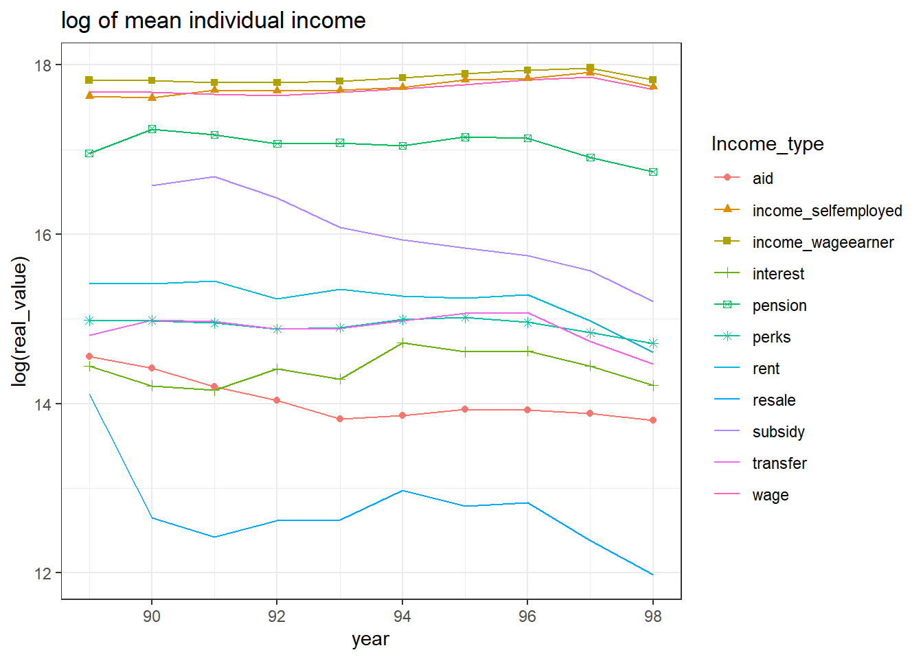
HH %>% select(wage_earning=income_w_y,self_employment=income_s_y, 
              pension=income_pension, rent=income_rent, interest=income_interest, 
              aid=income_aid, resale=income_resale, transfer=income_transfer,subsidy, 
              weight, cpi_y,year) %>%
  group_by(year) %>%
  summarize(across(wage_earning:subsidy,~weighted.mean(.x/cpi_y*100,weight,na.rm = T))) %>%
  pivot_longer(wage_earning:subsidy, names_to = "Income_type", values_to = "real_value") %>%
  ggplot(aes(x=year,y=log(real_value),color=Income_type,shape=Income_type)) +
  geom_line() + geom_point() + theme_bw() + ggtitle("log of mean houshold income")

HH %>% select(home_production=income_nm_miscellaneous, 
              homeownership=income_nm_house, public_service=income_nm_public,
              private_service=income_nm_private, agriculture=income_nm_agriculture, 
              nonagriculture=income_nm_nonagriculture, weight, cpi_y,year) %>%
  group_by(year) %>%
  summarize(across(home_production:nonagriculture,~weighted.mean(.x/cpi_y*100,weight,na.rm = T))) %>%
  pivot_longer(home_production:nonagriculture, names_to = "source", values_to = "real_value") %>%
  ggplot(aes(x=year,y=log(real_value),color=source,shape=source)) +
  geom_line() + geom_point() + theme_bw() + ggtitle("log of mean houshold non-monetary income")

## part 2 Tables
HH %>% group_by(year) %>%
  summarize(across(vehicle:microwave,~weighted.mean(.x,weight,na.rm = T)*100)) %>%
  pivot_longer(vehicle:microwave, names_to = "ownership", values_to = "value") %>%
  pivot_wider(ownership, names_from="year", values_from="value") %>%
  kable(caption = "Ownership of appliances") %>% 
  kable_styling("striped", "hover") %>%
  scroll_box(height = "500px")

Table 6.1: Ownership of appliances

ownership	89	90	91	92	93	94	95	96	97	98
vehicle	32.044086	34.287054	36.8242848	38.5299868	39.9944086	40.998873	42.2872882	45.4317331	48.1431199	48.2492697
motorcycle	21.504870	21.405463	20.2043174	19.1132713	18.9545103	19.097189	19.1934633	19.4219233	17.5772700	17.2208943
bicycle	10.924286	10.608479	10.6754941	9.0778261	8.9290592	9.655370	10.1027445	10.9412084	10.6668708	10.0941152
radio	4.742952	5.241358	4.9344468	5.3041197	4.9670771	6.061735	5.2442089	4.8055049	5.5518916	4.7050730
radiotape	31.895173	24.930207	19.4586475	12.2757186	10.5067684	11.258175	9.3820330	8.2453068	8.0037494	5.6882916
TVbw	1.305965	1.082868	0.8998664	0.7809093	0.8451319	0.702049	0.7177877	0.5651113	0.6385632	0.5066087
TV	96.182448	96.766413	97.3237603	97.3842163	97.5080115	97.582360	97.1455161	97.2621551	97.1292036	97.3949559
VHS_VCD_DVD	59.593567	59.025357	55.6182407	52.8989633	48.1923690	43.537587	37.7488667	32.2751922	28.4568865	22.4121013
computer	30.199864	30.890259	31.7840556	30.5757689	31.8352162	33.106736	31.4917813	31.6752240	28.0523015	25.5712235
cellphone	84.350495	86.695630	89.3213491	91.7183319	92.2684064	92.928764	93.2140438	94.1244588	94.7057709	94.7116372
freezer	24.445325	21.698493	23.9012590	20.3137289	19.5963365	18.492470	18.5894680	19.2659699	19.0047403	17.4673227
refridgerator	68.301990	65.067908	61.4027282	53.6005521	51.1731606	48.173513	46.5271099	43.0734899	38.2532346	36.1354766
fridge	33.731229	37.046642	40.7812408	47.8358973	50.8064348	53.929239	55.5674523	58.8469481	63.7913480	65.4624733
stove	97.270895	97.598102	97.9139542	97.9611886	98.5980975	98.447226	98.0934357	98.6501027	98.9712134	98.9308520
vacuum	77.460019	79.025143	80.4163027	81.2552060	82.8954632	82.902395	83.5286247	84.5298620	85.3129588	85.5423046
washingmachine	65.948230	68.448201	70.9885895	72.7930617	74.4796373	74.757089	76.1726414	78.3892720	79.1847071	79.7893007
sewingmachine	53.910737	50.417097	51.4890258	46.3400695	44.9010903	43.580851	44.1681375	43.7784552	41.5559165	42.2718729
fan	46.863772	47.472098	47.0207720	41.2225361	42.6021861	44.712986	44.3071327	42.3200337	40.9795287	40.4627640
evapcoolingportable	3.602268	4.129166	3.8455888	3.0525691	3.3280634	4.389036	5.3321325	4.7600827	5.7264126	6.5562657
splitportable	2.092733	2.163763	2.0110037	1.7633157	1.6596367	2.973040	3.1354347	2.9899434	9.5607524	9.7233895
dishwasher	1.710184	1.520522	2.4377892	3.2325146	3.9786541	4.225521	4.3475737	5.5743686	6.4808225	5.9354742
microwave	NaN	NaN	4.3076758	6.0683142	6.8848563	7.700641	8.0485029	9.8171794	10.0095190	9.9102724

HH %>% group_by(year) %>%
  summarize(across(pipewater:wastewater,~weighted.mean(.x,weight,na.rm = T)*100)) %>%
  pivot_longer(pipewater:wastewater, names_to = "Facilities", values_to = "value") %>%
  pivot_wider(Facilities, names_from="year", values_from="value") %>%
  kable(caption = "Usage of facilities and utilities") %>% 
  kable_styling("striped", "hover") %>%
  scroll_box(height = "500px")

Table 6.1: Usage of facilities and utilities

Facilities	89	90	91	92	93	94	95	96	97	98
pipewater	97.8785448	97.9130607	98.4710632	97.6265717	98.1272951	98.442079	98.4720568	98.4472712	98.223134	98.452090
electricity	99.8691970	99.8831778	99.9298740	99.8916748	99.9690206	99.978355	99.9810479	99.9796054	99.969377	99.984314
pipegas	78.3223284	79.1157120	81.0724332	81.4064838	82.9774731	84.270218	85.6867956	86.9416956	88.082540	89.248484
telephone	83.0497153	81.2992865	80.2274821	74.9571520	73.6896000	72.031910	70.5342963	68.3672583	63.497348	62.215469
internet	12.6857995	12.9691727	12.7475008	14.3161649	20.6185394	27.947556	34.9702771	46.3380861	51.064353	55.841567
bathroom	92.8538846	93.6542147	94.8153736	95.5067249	96.0755992	96.973625	97.3406737	97.6817778	97.537488	97.770370
kitchen	92.7014057	92.6727796	93.7739536	94.9355263	95.4203585	96.289655	96.4688741	96.8535643	96.746364	97.064488
evapcooling	51.9504903	51.5357049	53.5144524	52.7130350	52.8003160	53.462363	54.7791710	54.7452664	54.133939	53.838683
centralcooling	0.4756985	0.0926200	0.3145488	0.2417045	0.2363693	0.280906	0.3446441	0.3662051	1.614958	2.040089
centralheating	3.9045045	3.5679551	3.4620939	3.7985646	4.5095994	3.921872	3.3122853	4.0690850	4.889577	5.349666
package	0.9046314	0.7378605	0.9122994	2.5806133	3.2976652	4.274731	5.0126457	5.3153647	7.440690	8.200683
split	11.4852855	12.5263879	13.2354663	15.1816066	15.9254080	16.286405	17.2581213	18.6958676	14.872220	15.962490
wastewater	19.1754341	22.4744916	24.7278008	26.0863063	29.1130967	28.907997	31.3666964	33.1990240	32.643050	34.795353

HH %>% group_by(year) %>%
  summarize(across(celebration_m:occasions_other_y,~weighted.mean(.x,weight,na.rm = T)*100)) %>%
  pivot_longer(celebration_m:occasions_other_y, names_to = "Events", values_to = "value") %>%
  pivot_wider(Events, names_from="year", values_from="value") %>%
  kable(caption = "Percent of special occasions") %>% 
  kable_styling("striped", "hover") %>%
  scroll_box(height = "500px")

Table 6.1: Percent of special occasions

Events	89	90	91	92	93	94	95	96	97	98
celebration_m	0.6841955	0.6062397	0.7200362	0.5227151	0.3953824	0.4439151	0.6756492	NaN	NaN	NaN
celebration_y	8.7097186	6.8337356	6.2903440	5.1810402	4.3878037	4.0725063	4.2342948	NaN	NaN	NaN
mourning_m	0.3569481	0.2628881	0.3867271	0.2453985	0.2262652	0.3281505	0.3627335	NaN	NaN	NaN
mourning_y	4.9364529	4.3373832	3.7345113	3.0161507	2.9730448	2.5902881	2.6705856	NaN	NaN	NaN
house_maintenance_m	0.5716507	0.4078366	0.5905258	0.3541650	0.2407359	0.3676058	0.2982854	NaN	NaN	NaN
house_maintenance_y	18.9818650	14.7795837	13.7458350	12.9355498	12.5028331	13.7925323	11.9127170	NaN	NaN	NaN
pilgrimage_m	0.5065514	0.4033955	0.4999235	0.3797466	0.2792169	0.3317466	0.3887250	NaN	NaN	NaN
pilgrimage_y	4.7866841	5.3491242	4.1393377	3.8022088	3.8303963	3.5279654	4.2349734	NaN	NaN	NaN
travel_abroad_m	0.0614426	0.0436193	0.0504996	0.0096461	0.0307420	0.0470456	0.0199105	NaN	NaN	NaN
travel_abroad_y	0.7653344	0.7060629	0.3496505	0.3342689	0.3689184	0.4636468	0.4786188	NaN	NaN	NaN
surgery_m	1.3128234	7.4659919	1.0261479	0.8442002	0.7111846	0.7327604	1.1845466	NaN	NaN	NaN
surgery_y	NaN	NaN	8.4839387	10.2534603	10.0223565	10.1378510	11.4536563	NaN	NaN	NaN
occasions_other_m	0.1824038	0.2011443	0.0519317	0.1122528	0.0663388	0.0234342	0.0921761	NaN	NaN	NaN
occasions_other_y	1.4434763	1.2628412	1.0477819	0.9028352	0.9128925	0.7339645	1.3429496	NaN	NaN	NaN

HH %>% group_by(year, tenure) %>%
  summarize(number = sum(weight)) %>%
  group_by(year) %>%
  mutate(share = number/sum(number)*100) %>%
  pivot_wider(tenure, names_from="year", values_from="share") %>%
  kable(caption = "Type of land tenure") %>% 
  kable_styling("striped", "hover") %>%
  scroll_box(height = "300px")

Table 6.1: Type of land tenure

tenure	89	90	91	92	93	94	95	96	97	98
OwnedEstateLand	70.509826	71.9112625	72.4965948	68.5082156	70.2453572	71.2463715	70.8829332	70.2132045	68.5195650	70.9943861
OwnedEstate	0.460459	0.5058831	0.8442999	1.2626435	0.5667466	0.4496952	0.4745410	0.7462290	0.7791592	0.7332434
Rent	12.512256	12.8255755	11.9691409	13.9420839	13.0644895	13.1281141	12.8025961	12.5513282	13.0487088	11.8665090
Mortgage	6.159666	5.3485091	5.4054535	6.4215287	6.1370277	6.0557046	7.0420388	7.4787194	8.1184158	7.5853020
Service	1.865255	1.9975804	1.7681756	1.2975362	1.0589974	0.9191415	0.9599049	0.9439448	1.0119532	1.0289055
Free	8.469659	7.3911484	7.4557349	8.5110640	8.9165892	8.0804127	7.6595030	7.9608811	8.3280660	7.6845880
Other	0.022879	0.0200409	0.0606004	0.0569281	0.0107924	0.1205604	0.1784831	0.1056929	0.1941321	0.1070660

HH %>% group_by(year, material) %>%
  summarize(number = sum(weight)) %>%
  group_by(year) %>%
  mutate(share = number/sum(number)*100,
         material = fct_explicit_na(material, na_level = "Concrete/Metal")) %>%
  pivot_wider(material, names_from="year", values_from="share") %>%
  kable(caption = "Structure of construction") %>% 
  kable_styling("striped", "hover") %>%
  scroll_box(height = "300px")

Table 6.1: Structure of construction

material	89	90	91	92	93	94	95	96	97	98
MetalBlock	50.7487859	50.2823799	50.2805018	45.0873600	45.0127169	45.6227340	45.1298437	44.9034213	41.0373447	39.6361619
BrickWood	9.2253562	8.1992067	7.8001110	7.1512141	6.9948768	6.5600465	6.0090994	5.1489506	4.5170369	4.4998637
Cement	5.6019810	6.1838089	6.2032411	6.2924648	6.2019466	6.4606897	6.6011936	6.8967609	6.9855811	6.3647967
Brick	0.5284891	1.0752810	0.9108127	0.6688838	0.6041013	0.9494151	0.7717006	0.6187621	0.4116466	0.4429398
Wood	0.1172491	0.0981936	0.0996924	0.1150438	0.0784970	0.0435057	0.0297563	0.0329064	0.0480085	0.1399719
WoodKesht	3.9534235	3.8622777	3.4179404	2.5659179	2.5951111	2.3658098	2.3190851	2.2623997	1.8494649	1.5211601
KeshtGel	1.9755097	2.1057696	1.8874040	1.5579500	1.4102031	1.3254096	1.3512399	1.3184669	1.0748399	0.9721298
Other	1.6571423	1.5527438	1.7318665	3.2002048	3.2793974	2.2860894	1.9200372	1.5619829	1.6396876	1.4928485
Concrete/Metal	26.1920632	26.6403387	27.6684302	33.3609607	33.8231497	34.3863001	35.8680442	37.2563493	42.4363899	44.9301275

HH %>% group_by(year) %>%
  summarize(across(room:space,~weighted.mean(.x,weight,na.rm = T))) %>%
  kable(caption = "House characteristics") %>% 
  kable_styling("striped", "hover") %>%
  scroll_box(height = "400px")

Table 6.1: House characteristics

year	room	space
89	3.404627	92.64194
90	3.406734	93.43689
91	3.511407	95.19792
92	3.561369	93.30407
93	3.578862	93.62449
94	3.603388	94.02177
95	3.604649	94.93553
96	3.631116	95.02705
97	3.659141	96.04347
98	3.668576	95.78518

HH %>%  group_by(year, province) %>%
  summarize(car_ownership=weighted.mean(vehicle,weight)*100) %>%
  pivot_wider(province, names_from="year", values_from="car_ownership") %>%
  kable(caption = "Car ownership by province and year") %>% 
  kable_styling("striped", "hover") %>%
  scroll_box(height = "500px")

Table 6.1: Car ownership by province and year

province	89	90	91	92	93	94	95	96	97	98
Markazi	31.89084	34.71904	43.01038	39.15167	42.88604	42.13075	47.87688	46.83616	51.64630	49.57154
Gilan	22.97184	26.18817	28.31736	31.51883	32.77052	32.40062	31.82786	34.25897	36.47945	35.20249
Mazandaran	32.16812	28.61454	28.33231	35.43812	36.44276	39.69487	39.79995	45.61835	45.85421	43.52625
AzarbaijanSharghi	30.14212	30.86273	32.97825	37.50317	37.22126	36.57151	38.77929	39.48517	43.10528	43.27720
AzarbaijanGharbi	32.94096	34.18020	36.98186	41.78300	42.96266	47.62821	40.06852	45.50664	45.40959	54.73390
Kermanshah	23.97959	26.03655	27.94130	30.37149	32.39774	29.53845	30.79875	33.61177	43.05263	42.31064
Kouzestan	31.59621	29.53371	35.74085	35.52991	34.45655	32.42161	34.00649	38.74230	38.62614	40.07028
Fars	32.58198	35.68393	38.88914	38.76896	37.81940	41.40155	43.09984	46.08379	51.16417	48.51447
Kerman	41.86930	43.07374	43.93290	43.80613	38.69740	42.51203	47.94151	54.50490	55.01675	54.21379
KhorasanRazavi	30.08230	30.55565	33.87559	37.54692	38.68014	36.49834	39.16248	42.27683	45.79554	44.00599
Esfahan	39.17186	44.35660	42.49254	42.88777	47.57625	46.97424	48.97631	52.98739	58.29897	60.19234
SistanBalouchestan	18.56919	16.24629	17.18576	19.91114	18.87572	20.07803	21.06130	22.73198	28.23147	28.00504
Kordestan	21.00364	21.45523	22.40532	26.60195	28.66375	28.19885	31.54782	36.57922	37.55322	41.69228
Hamedan	28.38906	26.02956	30.10632	27.24881	30.27929	36.73583	39.63895	43.01405	43.48110	38.64652
CharmahalBakhtiari	29.05778	34.59619	34.66550	36.42123	40.51586	39.62012	44.89361	48.58939	50.50325	46.09934
Lorestan	24.29695	27.46413	28.83553	21.81317	27.93626	22.76006	22.88330	30.98613	31.61587	32.93983
Ilam	33.58796	33.56935	29.34788	33.40352	34.89885	33.36855	34.46365	38.83065	44.75097	44.21638
KohkilouyeBoyerahamad	28.22257	27.46634	24.37835	29.30624	28.78879	28.05718	21.60092	22.00725	29.49408	33.02894
Boushehr	36.44195	42.14790	42.87873	46.48129	50.24133	48.40139	50.57697	53.60981	59.71293	54.40757
Zanjan	29.89925	35.95433	35.24348	37.07151	36.83635	36.01768	32.35527	38.78832	42.13578	45.73873
Semnan	33.51018	35.27353	37.37244	43.67425	44.65979	42.84886	44.62168	47.87019	50.79232	52.66296
Yazd	57.39872	57.21516	60.37657	60.83035	62.06805	60.33636	62.36644	66.94192	70.21662	70.79475
Hormozgan	22.93388	29.90107	32.35488	34.98067	40.09436	41.67693	41.42824	42.76953	41.10113	39.64233
Tehran	36.32085	41.52333	45.49218	47.97036	50.56713	54.14764	55.27813	56.24781	58.57913	60.30397
Ardebil	24.56566	27.23159	30.43822	24.75731	26.35355	30.64916	31.02180	36.32265	35.08313	35.89254
Qom	28.18728	34.27098	36.03244	42.53090	44.26291	37.00672	48.31371	51.78613	51.77588	52.62781
Qazvin	33.17309	38.27826	39.96982	38.11254	34.95712	37.24503	37.40380	37.62343	45.94644	43.72430
Golestan	23.73958	28.89320	32.89236	30.24539	29.57864	31.97782	33.30858	36.58667	39.37090	39.30258
KhorasanShomali	20.79677	22.35501	24.54880	28.61405	31.60961	35.07212	36.57086	40.60135	41.42278	41.55714
KhorasanJonoubi	37.19021	37.96605	39.16171	42.48087	41.35287	43.29437	38.33531	44.96586	47.76810	49.45761
Alborz	NA	38.41375	40.27678	42.81827	49.35706	51.15320	52.03617	52.10986	54.43409	49.62397