Chapter 7 Trends in individual-level data

In this section, I present the trend of variables in the individual-level data.

library(tidyverse) 
library(knitr)
library(kableExtra)

rm(list = ls())

list_IND <- list.files(path = "./../exported", pattern = "^IND.*\\Rds$")

IND <- NULL
for (year in list_IND) {
  IND <- assign(year, readRDS(paste0("./../exported/",year))) %>% 
    filter(!is.na(weight)) %>%
    mutate(year = parse_number(year)) %>%
    bind_rows(IND)
  rm(list=year)
}

IND %>%
  mutate(literate = (literacy=="literate")*100,
         student = (studying=="Yes")*100,
         female = (gender=="Female")*100 ) %>%
  group_by(year) %>%
  summarize(across(c(khanevartype, literate, student, female, age, hours_w, days_w, hours_s, days_s),
                   ~weighted.mean(.x,weight,na.rm = T))) %>%
  pivot_longer(khanevartype:days_s, names_to = "Individual_characteristics", values_to = "value") %>%
  pivot_wider(Individual_characteristics, names_from="year", values_from="value") %>%
  kable(caption = "Trend of mean individual characteristics") %>% 
  kable_styling("striped", "hover") %>%
  scroll_box(height = "300px")

Table 7.1: Trend of mean individual characteristics

Individual_characteristics	89	90	91	92	93	94	95	96	97	98
khanevartype	1.001268	1.001268	1.001500	1.000587	1.000646	1.000365	1.001348	1.000713	1.001219	1.000926
literate	83.602879	83.316930	83.618546	85.242792	85.495947	85.490397	85.633596	86.345914	87.218438	87.325561
student	30.719317	30.657163	30.117890	29.329119	28.871824	28.668172	27.991695	27.376933	26.965645	26.180286
female	49.901832	50.031919	49.937203	49.603845	49.800529	49.919711	49.828943	49.909681	49.772406	50.002658
age	31.214607	31.932403	32.660355	31.450977	32.249490	32.776086	33.286370	33.497837	33.214002	34.184482
hours_w	8.512224	8.536169	8.514653	8.426629	8.413178	8.443573	8.415468	8.540553	8.567393	8.535429
days_w	5.578062	5.610158	5.553329	5.562511	5.568581	5.555247	5.508658	5.534698	5.574768	5.593744
hours_s	7.725828	7.749941	7.845208	7.832617	7.740324	7.815028	7.761225	7.937650	8.024436	7.937381
days_s	6.501877	6.402398	6.432165	6.388551	6.396116	6.337979	6.249191	6.267626	6.210391	6.234992

IND %>% group_by(year, education) %>%
  summarize(number = sum(weight)) %>%
  group_by(year) %>%
  mutate(share = number/sum(number)*100) %>%
  pivot_wider(education, names_from="year", values_from="share") %>%
  kable(caption = "Trend of education-level") %>% 
  kable_styling("striped", "hover") %>%
  scroll_box(height = "300px")

Table 7.1: Trend of education-level

education	89	90	91	92	93	94	95	96	97	98
Elemantry	27.4179293	26.9558956	27.3383235	27.3431344	27.4436532	27.5148864	27.4352938	27.0558504	25.8042373	25.6667534
Secondary	15.9497885	16.2280615	15.6610064	15.1920500	14.2881366	14.8987009	15.1181891	15.2680867	15.5019227	15.4230765
HighSchool	4.9248632	4.5006534	4.3578238	4.6338828	5.4099959	4.7036006	4.4113239	4.1121194	4.1299510	4.2677753
Diploma	15.6913560	15.7270475	15.8424642	15.1835181	16.1720745	16.3517987	16.4026533	17.0096987	17.2682861	17.6466180
College	3.2418831	3.3760137	3.3154985	3.3470578	3.5061038	3.5078284	3.4729789	3.4734857	3.5672502	3.4931683
Bachelor	8.0135856	8.3270709	8.9204476	9.3472453	9.2292317	9.1854107	9.2927006	9.6921996	9.7624141	10.0362701
Master	0.7105265	0.9649471	1.2293105	1.3908550	1.7759496	1.9737183	2.2272200	2.3862066	2.6228452	2.6540900
PhD	0.1130590	0.0700451	0.0742135	0.1039445	0.1363366	0.1941889	0.2469767	0.2438966	0.1337045	0.2363086
Other	0.6872334	0.6036479	0.6531497	0.5642147	NA	NA	NA	NA	0.5275625	0.5018630
NA	23.2497755	23.2466174	22.6077623	22.8940971	22.0385183	21.6698673	21.3926636	20.7584563	20.6818264	20.0740768

IND %>% group_by(year, education) %>%
  summarize(number = sum(weight)) %>%
  group_by(year) %>%
  mutate(share = number/sum(number)) %>%
  ggplot(aes(x=year,y=share,fill=education)) + 
  geom_col() +
  #geom_text(aes(label = scales::percent(share)), position = position_stack(vjust = 0.5)) + 
  theme_bw() 

IND %>% group_by(year, relation) %>%
  summarize(number = sum(weight)) %>%
  group_by(year) %>%
  mutate(share = number/sum(number)*100) %>%
  pivot_wider(relation, names_from="year", values_from="share") %>%
  kable(caption = "Trend of relationship with houshold head") %>% 
  kable_styling("striped", "hover") %>%
  scroll_box(height = "400px")

Table 7.1: Trend of relationship with houshold head

relation	89	90	91	92	93	94	95	96	97	98
Head	26.3254514	26.6112215	27.0900754	28.0990164	28.3246302	28.4575214	28.7046541	28.7849908	29.3539703	29.5364925
Spouse	22.1063708	22.2137142	22.4996692	23.8397578	23.7604768	23.7842859	23.9314996	24.1297725	24.4905686	24.5092192
Child	47.1016528	47.0020117	46.3588156	44.8672394	44.5858656	44.5406326	44.0449584	43.8862288	42.8234469	42.7469844
SonDaughter_inLaw	1.0269177	1.0047514	0.9515441	0.6938261	0.7256086	0.6875495	0.7026408	0.6418243	0.5705477	0.5291946
GrandSonDaughter	1.2106559	1.1652605	1.1639143	0.9391639	0.9971313	1.0545372	1.0750574	1.0975951	1.1462817	1.1289256
Parent	0.9369964	0.8812030	0.8859965	0.7773839	0.7733104	0.7433376	0.7593385	0.7414480	0.7834874	0.7283398
Sibling	0.7182855	0.5961798	0.5676886	0.4439059	0.5052952	0.4001753	0.4669795	0.4339498	0.4395565	0.4564733
OtherRelative	0.4125645	0.3831132	0.3485921	0.2758895	0.2420757	0.2124597	0.2516056	0.2315500	0.3098134	0.2963955
NonRelative	0.1611050	0.1425447	0.1337041	0.0638170	0.0856063	0.1195007	0.0632661	0.0526406	0.0823275	0.0679750

IND %>% group_by(year, maritalst) %>%
  summarize(number = sum(weight)) %>%
  group_by(year) %>%
  mutate(share = number/sum(number)*100) %>%
  pivot_wider(maritalst, names_from="year", values_from="share") %>%
  kable(caption = "Trend of marital status") %>% 
  kable_styling("striped", "hover") %>%
  scroll_box(height = "200px")

Table 7.1: Trend of marital status

maritalst	89	90	91	92	93	94	95	96	97	98
Married	49.0326918	49.111976	49.715671	51.3841124	51.261460	51.151987	51.338463	51.660369	52.041044	52.002669
Widowed	3.9631069	4.197008	4.282663	3.8590685	4.184238	4.133063	4.332200	4.187647	4.221930	4.306677
Divorced	0.7910894	0.894192	1.037142	0.8897502	1.075377	1.229318	1.219983	1.264830	1.430927	1.440146
Single	32.6162394	32.741118	32.264639	28.5834258	28.683464	29.124115	29.016093	28.721138	27.065574	27.679812
NA	13.5968726	13.055705	12.699885	15.2836432	14.795462	14.361517	14.093261	14.166015	15.240526	14.570697

IND %>% group_by(year, occupationalst) %>%
  summarize(number = sum(weight)) %>%
  group_by(year) %>%
  mutate(share = number/sum(number)*100) %>%
  pivot_wider(occupationalst, names_from="year", values_from="share") %>%
  kable(caption = "Trend of employment status") %>% 
  kable_styling("striped", "hover") %>%
  scroll_box(height = "300px")

Table 7.1: Trend of employment status

occupationalst	89	90	91	92	93	94	95	96	97	98
employed	28.513920	27.585573	28.335838	28.183325	27.728575	27.465109	27.324447	27.761092	27.789235	27.250272
unemployed	5.298381	5.816293	5.682773	4.759909	4.904475	5.274785	5.626695	5.349918	5.002252	5.173184
IncomeWOJob	8.506198	8.658578	9.018800	8.499383	9.349279	9.236707	9.536829	9.723449	9.690237	10.491756
Student	17.483612	17.779308	17.243620	15.964403	15.725067	15.742607	15.473114	15.215887	14.804962	14.535477
Housewife	24.350677	24.826701	24.817637	25.414939	25.441029	25.870279	25.876333	25.697787	25.646267	26.045687
Other	2.250010	2.273938	2.200392	1.891518	2.056112	2.043811	2.068338	2.085853	1.820692	1.932469
NA	13.597203	13.059609	12.700940	15.286523	14.795462	14.366701	14.094243	14.166015	15.246355	14.571155

IND %>% group_by(year, status_w) %>%
  summarize(number = sum(weight)) %>%
  group_by(year) %>%
  mutate(share = number/sum(number)*100) %>%
  pivot_wider(status_w, names_from="year", values_from="share") %>%
  kable(caption = "Trend of job-status of wage-earners") %>% 
  kable_styling("striped", "hover") %>%
  scroll_box(height = "200px")

Table 7.1: Trend of job-status of wage-earners

status_w	89	90	91	92	93	94	95	96	97	98
public	4.2575349	3.9216423	4.1921650	4.166793	3.983877	3.8425475	3.9190328	3.9622387	3.8090221	3.7287082
cooperative	0.0707955	0.0665362	0.0575354	0.050287	0.050758	0.0478215	0.0239547	0.0364969	0.0426843	0.0240996
private	13.6524155	12.8585388	13.0103767	13.343096	13.798232	13.9974171	13.9940446	14.5115773	14.4381913	14.0669243
NA	82.0192541	83.1532827	82.7399229	82.439824	82.167133	82.1122139	82.0629679	81.4896871	81.7101023	82.1802679

IND %>% group_by(year, status_s) %>%
  summarize(number = sum(weight)) %>%
  group_by(year) %>%
  mutate(share = number/sum(number)*100) %>%
  pivot_wider(status_s, names_from="year", values_from="share") %>%
  kable(caption = "Trend of job-status of self-employment") %>% 
  kable_styling("striped", "hover") %>%
  scroll_box(height = "200px")

Table 7.1: Trend of job-status of self-employment

status_s	89	90	91	92	93	94	95	96	97	98
employer	1.997396	1.735552	1.707096	1.574974	1.344553	1.156768	1.276251	1.239464	1.234822	1.145904
selfemployed	9.080730	8.834283	9.085923	8.987861	8.695944	9.012654	9.002299	9.148716	9.295213	9.351290
familyworker	2.749234	2.435735	2.507786	2.007001	1.869709	1.627454	1.380053	1.177641	1.123499	1.164581
NA	86.172640	86.994431	86.699195	87.430165	88.089794	88.203125	88.341397	88.434179	88.346466	88.338225

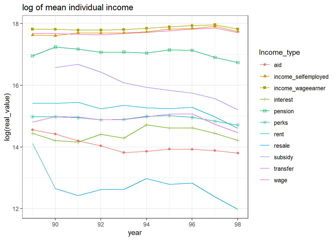
IND %>% select(income_wageearner=income_w_y,wage=wage_w_y, perks=perk_w_y,income_selfemployed=income_s_y,
              pension=income_pension, rent=income_rent, interest=income_interest, 
              aid=income_aid, resale=income_resale, transfer=income_transfer,subsidy, 
              weight, cpi_y,year) %>%
  group_by(year) %>%
  summarize(across(income_wageearner:subsidy,~weighted.mean(.x/cpi_y*100,weight,na.rm = T))) %>%
  pivot_longer(income_wageearner:subsidy, names_to = "Income_type", values_to = "real_value") %>%
  ggplot(aes(x=year,y=log(real_value),color=Income_type,shape=Income_type)) +
  geom_line() + geom_point() + theme_bw() + ggtitle("log of mean individual income")

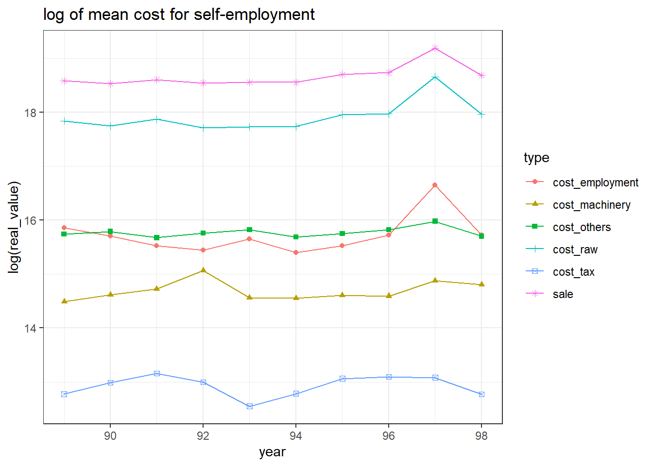
IND %>% select(cost_employment:sale,weight, cpi_y,year) %>%
  group_by(year) %>%
  summarize(across(cost_employment:sale,~weighted.mean(.x/cpi_y*100,weight,na.rm = T))) %>%
  pivot_longer(cost_employment:sale, names_to = "type", values_to = "real_value") %>%
  ggplot(aes(x=year,y=log(real_value),color=type,shape=type)) +
  geom_line() + geom_point() + theme_bw() + ggtitle("log of mean cost for self-employment")