Chapter 4 Cleaning data
The raw data (in rdata format) consists of several data frames corresponding to the questionnaire tables. Each data frame’s name informs the user about the region, year, part, and table number. For example, R98P3S01 contains Table 1 (food) of Part 3 (expenditure item) for the R (rural) sample of year 98. My data cleaning process has different steps:
- for each year of the survey, I write a script to reconcile variable names and codings.
- I match item codes with detailed price index
- I merge different rounds and build household and individual level datasets over time.
This chapter describes the script structure for each survey year and presents a sample code written for 1398. The output of each script, in addition to the cleaned raw data, would be three .RDS files (which can be easily exported to .csv, .dta, and other formats) including (1) household-level, (2) individual-level, (3) item-level data frames. For example, the script of the 1398 survey, takes the raw data of 98.Rdata file as input and creates the following 4 files as output:
- HEIS98.Rdata which is a cleaned image of the data
- HH98.Rds which is the household-level data
- IND98.Rds which is the individual-level data
- EXP98.Rds which is the item-level data
The year-wise scripts can be downloaded from here: https://github.com/m-hoseini/HEIS_script
The cleaned data files for each can be downloaded from here: https://b2n.ir/d12374
In each yearly scripts, I do the following steps:
- rename variable to have unique names over time
- recode expenditure items to have global code over time
- attaching each expenditure item to its corresponding price index
- merging tables of part 3 to build a unique expenditure data frame
- merging part 1 and part 4 to build individual-level data on characteristics and income
- aggregating expenditures and income to make household-level data
4.1 Importing raw data and sampling information
In the first step, I import tidyverse library, clear the memory, and import the raw data. In most years, raw data has a separate file for information about the sample, like whether it is the original household in the framework, the sample weight, etc. In this code, first, I define province labels, and the last two lines regarding Part 1 are for generating variables for province and town codes. The information on the location is available in household ID variables titled “Address” in the surveys. The structure of Address is changing over time and I explain it later.
library(tidyverse)

rm(list = ls())

load("./RAW/98.RData")

##############################
Province <- c(Markazi="00", Gilan="01", Mazandaran="02", AzarbaijanSharghi="03", AzarbaijanGharbi="04",
              Kermanshah="05", Kouzestan="06", Fars="07", Kerman="08", KhorasanRazavi="09",
              Esfahan="10", SistanBalouchestan="11", Kordestan="12", Hamedan="13", CharmahalBakhtiari="14",
              Lorestan="15", Ilam="16", KohkilouyeBoyerahamad="17", Boushehr="18", Zanjan="19",
              Semnan="20", Yazd="21", Hormozgan="22", Tehran="23", Ardebil="24", Qom="25", Qazvin="26",
              Golestan="27", KhorasanShomali="28", KhorasanJonoubi="29", Alborz="30")

R98Data <- R98Data %>%
  rename(month = MahMorajeh, khanevartype = NoeKhn) %>%
  mutate(province = fct_recode(as.factor(substr(Address, 2, 3)), !!!Province),
         town = as.integer(substr(Address, 4, 5)))
U98Data <- U98Data %>%
  rename(month = MahMorajeh, khanevartype = NoeKhn) %>%
  mutate(province = fct_recode(as.factor(substr(Address, 2, 3)), !!!Province),
         town = as.integer(substr(Address, 4, 5)))
4.2 Cleaning Part 1
For part 1, I first define my global codes for member characteristics, including relation, gender, literacy, studying, education, occupation, and marital status, such that these variables become comparable over time. Then I change variable names to have unique names over time. The below code shows the name list of 1398. Finally, I assign my global value labels of the variables (levels of factors).
4.2.1 Education code
Education coding has been changing time to time in HEIS. Between 1376 and 1384, it is reported based on a 2-digit detailed coding. Then, from 1385 to 1392, the coding changed to conform to 3-digit International Standard Classification of Education (ISCED-97). Afterward, it was reclassified to a 1-digit code, and then slightly modified in 1397. The global coding of education includes the below groups:
- Elemantry (up to primary school/ adult literacy program ابتدایی/سوادآموزی )
- Secondary school (راهنمایی/متوسطه۱)
- High school (متوسطه/متوسطه۲)
- Diploma (دیپلم و پیشدانشگاهی)
- College (فوقدیپلم/کاردانی)
- Bachelor (لیسانس/کارشناسی)
- Master (کارشناسی ارشد و دکترای حرفهای)
- PhD (دکتری تخصصی)
- Others/informal (سایر و غیر رسمی)
Based on the HEIS manual, for students, the education code represents their current studying degree, but for non-students, it corresponds to the last degree they finished. In this regards, code 3 (High school) can be only given to students and non-student who finish only some years of highschool are labeled by code 2. Between 1393 and 1396, literates who completed “adult literacy program” belonged to the last group (“others/informal”), but after 1397 they classified as “elemantary.” Their population is 3 to 4 times higher than others groups within “others/informal” before 1393, but between 1393 and 1396, they cannot be distinguished from other groups in last code (“others/informal”). Thus, to have a unique and consistent code over time, between 1393 and 1396, we classify all individuals with education code “others/informal” as “elementary.”
##############################
# Part 1

relation <- c(Head="1", Spouse="2", Child="3", SonDaughter_inLaw="4", GrandSonDaughter="5", Parent="6", Sibling="7", OtherRelative="8", NonRelative="9")
gender <- c(Male="1", Female="2")
literacy <- c(literate="1", illiterate="2")
yesno <- c(Yes="1", No="2")
education <- c(Elemantry="1", Secondary="2", HighSchool="3", Diploma="4", College="5", Bachelor="6", Master="7", PhD="8", Other="9")
occupation <- c(employed="1", unemployed="2", IncomeWOJob="3", Student="4", Housewife="5", Other="6")
marital <- c(Married ="1", Widowed="2", Divorced="3", Single="4")

R98P1 <- R98P1 %>%
  rename(
    member = DYCOL01,
    relation = DYCOL03,
    gender = DYCOL04,
    age = DYCOL05,
    literacy = DYCOL06,
    studying = DYCOL07,
    degree = DYCOL08,
    occupationalst = DYCOL09,
    maritalst = DYCOL10) %>%
  mutate(across(where(is.character), as.integer),
         across(c(relation,gender,literacy,studying,degree,occupationalst,maritalst), as.factor),
         relation = fct_recode(relation, !!!relation),
         gender = fct_recode(gender, !!!gender),
         literacy = fct_recode(literacy, !!!literacy),
         studying = fct_recode(studying, !!!yesno),
         degree = fct_recode(degree, !!!education),
         occupationalst = fct_recode(occupationalst, !!!occupation),
         maritalst = fct_recode(maritalst, !!!marital))

U98P1 <- U98P1 %>%
  rename(
    member = DYCOL01,
    relation = DYCOL03,
    gender = DYCOL04,
    age = DYCOL05,
    literacy = DYCOL06,
    studying = DYCOL07,
    degree = DYCOL08,
    occupationalst = DYCOL09,
    maritalst = DYCOL10 ) %>%
  mutate(across(where(is.character), as.integer),
         across(c(relation,gender,literacy,studying,degree,occupationalst,maritalst), as.factor),
         relation = fct_recode(relation, !!!relation),
         gender = fct_recode(gender, !!!gender),
         literacy = fct_recode(literacy, !!!literacy),
         studying = fct_recode(studying, !!!yesno),
         degree = fct_recode(degree, !!!education),
         occupationalst = fct_recode(occupationalst, !!!occupation),
         maritalst = fct_recode(maritalst, !!!marital))
4.3 Cleaning Part 2
Cleaning Part 2 is similar to Part 1. First defining global labels for variables, then renaming the variables and assigning the labels to variables. Because many variables in this part are yes-no questions, I change the format of those variables to binary for saving space. Note that item “microwave” is added to after 1391 to this part. Also, the information regarding the special events (celebration, …) is reported in the raw data from 1384 to 1395.
##############################
# Part 2

tenure <- c(OwnedEstateLand="1", OwnedEstate="2", Rent="3", Mortgage="4", Service="5", Free="6", Other="7")
material <- c(MetalBlock="1", BrickWood="2", Cement="3", Brick="4", Wood="5", WoodKesht="6", KeshtGel="7", Other="8")
fuel <- c(Oil="1", Gasoline="2", LiquidGas="3", NaturalGas="4", Electricity="5", Wood="6", AnimalOil="7", Coke="8", Other="9", None="10" )
fuel1 <- c(Oil="11", Gasoline="12", LiquidGas="13", NaturalGas="14", Electricity="15", Wood="16", AnimalOil="17", Coke="18", Other="19", None="20" )
fuel2 <- c(Oil="21", Gasoline="22", LiquidGas="23", NaturalGas="24", Electricity="25", Wood="26", AnimalOil="27", Coke="28", Other="29", None="30" )

R98P2 <- R98P2 %>%
  rename(
    tenure = DYCOL01,
    room = DYCOL03,
    space = DYCOL04,
    construction = DYCOL05,
    material = DYCOL06,
    vehicle = DYCOL07,
    motorcycle = DYCOL08,
    bicycle = DYCOL09,
    radio = DYCOL10,
    radiotape = DYCOL11,
    TVbw = DYCOL12,
    TV = DYCOL13,
    VHS_VCD_DVD = DYCOL14,
    computer = DYCOL15,
    cellphone = DYCOL16,
    freezer = DYCOL17,
    refridgerator = DYCOL18,
    fridge = DYCOL19,
    stove = DYCOL20,
    vacuum = DYCOL21,
    washingmachine = DYCOL22,
    sewingmachine = DYCOL23,
    fan = DYCOL24,
    evapcoolingportable = DYCOL25,
    splitportable = DYCOL26,
    dishwasher = DYCOL27,
    microwave = DYCOL28,
    none = DYCOL29,
    pipewater = DYCOL30,
    electricity = DYCOL31,
    pipegas = DYCOL32,
    telephone = DYCOL33,
    internet  = DYCOL34,
    bathroom = DYCOL35,
    kitchen = DYCOL36,
    evapcooling = DYCOL37,
    centralcooling = DYCOL38,
    centralheating = DYCOL39,
    package = DYCOL40,
    split = DYCOL41,
    wastewater = DYCOL42,
    cookingfuel = DYCOL43,
    heatingfuel = DYCOL44,
    waterheatingfuel = DYCOL45) %>%
  mutate(across(where(is.character), as.integer),
         across(c(tenure,material,cookingfuel,heatingfuel,waterheatingfuel), as.factor),
         tenure = fct_recode(tenure, !!!tenure),
         material = fct_recode(material, !!!material),
         cookingfuel = fct_recode(cookingfuel, !!!fuel),
         heatingfuel = fct_recode(heatingfuel, !!!fuel1),
         waterheatingfuel = fct_recode(waterheatingfuel, !!!fuel2),
         across(vehicle:wastewater, ~!is.na(.x)))


U98P2 <- U98P2 %>%
  rename(
    tenure = DYCOL01,
    room = DYCOL03,
    space = DYCOL04,
    construction = DYCOL05,
    material = DYCOL06,
    vehicle = DYCOL07,
    motorcycle = DYCOL08,
    bicycle = DYCOL09,
    radio = DYCOL10,
    radiotape = DYCOL11,
    TVbw = DYCOL12,
    TV = DYCOL13,
    VHS_VCD_DVD = DYCOL14,
    computer = DYCOL15,
    cellphone = DYCOL16,
    freezer = DYCOL17,
    refridgerator = DYCOL18,
    fridge = DYCOL19,
    stove = DYCOL20,
    vacuum = DYCOL21,
    washingmachine = DYCOL22,
    sewingmachine = DYCOL23,
    fan = DYCOL24,
    evapcoolingportable = DYCOL25,
    splitportable = DYCOL26,
    dishwasher = DYCOL27,
    microwave = DYCOL28,
    none = DYCOL29,
    pipewater = DYCOL30,
    electricity = DYCOL31,
    pipegas = DYCOL32,
    telephone = DYCOL33,
    internet  = DYCOL34,
    bathroom = DYCOL35,
    kitchen = DYCOL36,
    evapcooling = DYCOL37,
    centralcooling = DYCOL38,
    centralheating = DYCOL39,
    package = DYCOL40,
    split = DYCOL41,
    wastewater = DYCOL42,
    cookingfuel = DYCOL43,
    heatingfuel = DYCOL44,
    waterheatingfuel = DYCOL45) %>%
  mutate(across(where(is.character), as.integer),
         across(c(tenure,material,cookingfuel,heatingfuel,waterheatingfuel), as.factor),
         tenure = fct_recode(tenure, !!!tenure),
         material = fct_recode(material, !!!material),
         cookingfuel = fct_recode(cookingfuel, !!!fuel),
         heatingfuel = fct_recode(heatingfuel, !!!fuel1),
         waterheatingfuel = fct_recode(waterheatingfuel, !!!fuel2),
         across(vehicle:wastewater, ~!is.na(.x)))
4.4 Cleaning Part 3
The most cumbersome step to clean HEIS is to match expenditure item data over time and adjust the value by price indices. I first rename all columns to have the same name over different rounds of surveys and then define a unique code for each expenditure item. As expenditure categories are changing over time and in many cases, a more general classification is decomposed into different categories, my global codes cover both general and detailed classifications. For example in one year there is an expenditure item ‘fruit’ and in the next year, it is decomposed into ‘apple,’ ‘banana,’ and other fruits. I then would have 4 global codes: 1-fruit, 2-apple, 3-banana, 4-other fruits.
4.4.1 Price index and real expenditure
After defining the global codes for each round, I merge each item with its price index. The index I use is based on an item-level monthly consumer price index published for over 500 items by the Central Bank of Iran. I obtained the indices for two base years: The index with the base year 1390 = 100, is available for years before 1395, and the index with the base year 1395 = 100, is available from 1392 onwards. I use the first index for the year before 1395, and the second index for years after 1395. To remove the drop in the level of indices between the two series, I compute the average ratio of the two indices in their overlapping years (1392 to 1395) for each item and multiply the second series by that ratio.
As the item coding in HEIS (COICOP) is different from CPI item code, I need to match each COICOP item to a proper CPI item. This correspondence is not always straightforward. Some COICOP items are corresponding to multiple CPI items and vice versa. For this reason, I compute the price index for each COICOP item as the weighted average of the index of its corresponding CPI items, where the weight is drawn from the base basket of CPI. Also, in several instances, there is no specific CPI code for a COICOP item (e.g. donations) and in these cases, I use overall CPI as the price index. Doing these steps result in a price index file (CPI.rds) in which a monthly price index is computed for each global code (COICOP item).
Because households are surveyed in different months of the year, and each table has a different recall period, for performing price adjustment of values, I note both the month of the survey and the recall period of the item. For items with past month recall period (Expenditure tables 1 to 12), I use the monthly price index, but for items with past year recall period (Expenditure tables 13 and 14), I use the average of the price index in 12 months ending to the month of the survey. Before 1387, the month of survey is not reported in the surveys and thus for these years I use the average price index in the corresponding year for each item.
Here is a sample code for 1398. At first, I define two data frames month that attaches the month of the survey to each household Address, and CPI which provides the COICOP-level monthly price index. Then for each table, I rename variables and define the unique item code as DYCOL00. Notice that the variables in all tables are not the same. The two variables “code” referring to item code in that year and “purchased” refers to the method of obtaining exist in all tables. But many variables exist in only some tables like “gram,” “kilogram,” “price” in tables 1 and 2, “cost” and “sell” in tables 13 and 14. In tables 1 to 12, “value” refers to the value of transactions, but in tables 13 and 14 no such variable already exists, and I define “value” as the net expenditure (cost - sell). I define a variable table to simplify summarizing expenditures in the next steps. The last four lines of code for each table is to merge the price index and to generate the value of expenditure in fixed price “value_r.” As mentioned above, in tables 1 to 12, the monthly price index is used, but in tables 13 and 14, the yearly average of the indices.
# Adding Global variable as DYCOL00

##############################
# Part 3, Table 1

month <- R98Data %>%
  bind_rows(U98Data) %>%
  select(Address,month) %>%
  mutate(year=1398)

CPI <- readRDS("CPI/CPI.rds")

R98P3S01 <- R98P3S01 %>%
  rename(
    code = DYCOL01,
    purchased = DYCOL02,
    gram = DYCOL03,
    kilogram = DYCOL04,
    price = DYCOL05,
    value = DYCOL06 ) %>%
  mutate(DYCOL00 = case_when(
    code == 11241 ~ 11240L,
    TRUE ~ code),
    across(c(price,value,kilogram),  ~ as.numeric(as.character(.x)) ),
    table = 1L) %>%
  left_join(month) %>%
  left_join(CPI) %>%
  mutate(value_r=value*100/cpi) %>%
  select(Address:table, value_r)


U98P3S01 <- U98P3S01 %>%
  rename(
    code = DYCOL01,
    purchased = DYCOL02,
    gram = DYCOL03,
    kilogram = DYCOL04,
    price = DYCOL05,
    value = DYCOL06 ) %>%
  mutate(DYCOL00 = case_when(
    code == 11241 ~ 11240L,
    TRUE ~ code),
    across(c(price,value,kilogram),  ~ as.numeric(as.character(.x)) ),
    table = 1L) %>%
  left_join(month) %>%
  left_join(CPI) %>%
  mutate(value_r=value*100/cpi) %>%
  select(Address:table, value_r)

# Part 3, Table 2
R98P3S02 <- R98P3S02 %>%
  rename(
    code = DYCOL01,
    purchased = DYCOL02,
    gram = DYCOL03,
    kilogram = DYCOL04,
    price = DYCOL05,
    value = DYCOL06 ) %>%
  mutate(DYCOL00 = code,
         table = 2L) %>%
  left_join(month) %>%
  left_join(CPI) %>%
  mutate(value_r=value*100/cpi) %>%
  select(Address:table, value_r)

U98P3S02 <- U98P3S02 %>%
  rename(
    code = DYCOL01,
    purchased = DYCOL02,
    gram = DYCOL03,
    kilogram = DYCOL04,
    price = DYCOL05,
    value = DYCOL06 ) %>%
  mutate(DYCOL00 = code,
         table = 2L) %>%
  left_join(month) %>%
  left_join(CPI) %>%
  mutate(value_r=value*100/cpi) %>%
  select(Address:table, value_r)

# Part 3, Table 3
R98P3S03 <- R98P3S03 %>%
  rename(
    code = DYCOL01,
    purchased = DYCOL02,
    value = DYCOL03 ) %>%
  mutate(DYCOL00 = case_when(
    code == 31244 ~ 31255L,
    code == 31269 ~ 31263L,
    TRUE ~ code),
    table = 3L) %>%
  left_join(month) %>%
  left_join(CPI) %>%
  mutate(value_r=value*100/cpi) %>%
  select(Address:table, value_r)


U98P3S03 <- U98P3S03 %>%
  rename(
    code = DYCOL01,
    purchased = DYCOL02,
    value = DYCOL03) %>%
  mutate(DYCOL00 = case_when(
    code == 31244 ~ 31255L,
    code == 31269 ~ 31263L,
    TRUE ~ code),
    table = 3L) %>%
  left_join(month) %>%
  left_join(CPI) %>%
  mutate(value_r=value*100/cpi) %>%
  select(Address:table, value_r)


# Part 3, Table 4
R98P3S04 <- R98P3S04 %>%
  rename(
    code = DYCOL01,
    mortgage = DYCOL02,
    purchased = DYCOL03,
    value = DYCOL04 ) %>%
  mutate(DYCOL00 = case_when(
    code == 44418 ~ 44419L,
    TRUE ~ code),
    table = 4L) %>%
  left_join(month) %>%
  left_join(CPI) %>%
  mutate(value_r=value*100/cpi) %>%
  select(Address:table, value_r)


U98P3S04 <- U98P3S04 %>%
  rename(
    code = DYCOL01,
    mortgage = DYCOL02,
    purchased = DYCOL03,
    value = DYCOL04 ) %>%
  mutate(DYCOL00 = case_when(
    code == 44418 ~ 44419L,
    TRUE ~ code),
    table = 4L)  %>%
  left_join(month) %>%
  left_join(CPI) %>%
  mutate(value_r=value*100/cpi) %>%
  select(Address:table, value_r)

# Part 3, Table 5
R98P3S05 <- R98P3S05 %>%
  rename(
    code = DYCOL01,
    purchased = DYCOL02,
    value = DYCOL03 ) %>%
  mutate(DYCOL00 = code,
         table = 5L) %>%
  left_join(month) %>%
  left_join(CPI) %>%
  mutate(value_r=value*100/cpi) %>%
  select(Address:table, value_r)


U98P3S05 <- U98P3S05 %>%
  rename(
    code = DYCOL01,
    purchased = DYCOL02,
    value = DYCOL03 ) %>%
  mutate(DYCOL00 = code,
         table = 5L) %>%
  left_join(month) %>%
  left_join(CPI) %>%
  mutate(value_r=value*100/cpi) %>%
  select(Address:table, value_r)


# Part 3, Table 6
R98P3S06 <- R98P3S06  %>%
  rename(
    code = DYCOL01,
    purchased = DYCOL02,
    value = DYCOL03) %>%
  mutate(DYCOL00 = case_when(
    code == 62128 ~ 62125L,
    code == 62129 ~ 62126L,
    TRUE ~ code),
    table = 6L) %>%
  left_join(month) %>%
  left_join(CPI) %>%
  mutate(value_r=value*100/cpi) %>%
  select(Address:table, value_r)


U98P3S06 <- U98P3S06 %>%
  rename(
    code = DYCOL01,
    purchased = DYCOL02,
    value = DYCOL03) %>%
  mutate(DYCOL00 = case_when(
    code == 62128 ~ 62125L,
    code == 62129 ~ 62126L,
    TRUE ~ code),
    table = 6L) %>%
  left_join(month) %>%
  left_join(CPI) %>%
  mutate(value_r=value*100/cpi) %>%
  select(Address:table, value_r)


# Part 3, Table 7
R98P3S07 <- R98P3S07 %>%
  rename(
    code = DYCOL01,
    purchased = DYCOL02,
    value = DYCOL03) %>%
  mutate(DYCOL00 = case_when(
    code == 73611 ~ 73615L,
    TRUE ~ code),
    table = 7L) %>%
  left_join(month) %>%
  left_join(CPI) %>%
  mutate(value_r=value*100/cpi) %>%
  select(Address:table, value_r)


U98P3S07 <- U98P3S07 %>%
  rename(
    code = DYCOL01,
    purchased = DYCOL02,
    value = DYCOL03 ) %>%
  mutate(DYCOL00 = case_when(
    code == 73611 ~ 73615L,
    TRUE ~ code),
    table = 7L) %>%
  left_join(month) %>%
  left_join(CPI) %>%
  mutate(value_r=value*100/cpi) %>%
  select(Address:table, value_r)


# Part 3, Table 8
R98P3S08 <- R98P3S08 %>%
  rename(
    code = DYCOL01,
    purchased = DYCOL02,
    value = DYCOL03) %>%
  mutate(DYCOL00 = code,
         table = 8L) %>%
  left_join(month) %>%
  left_join(CPI) %>%
  mutate(value_r=value*100/cpi) %>%
  select(Address:table, value_r)


U98P3S08 <- U98P3S08 %>%
  rename(
    code = DYCOL01,
    purchased = DYCOL02,
    value = DYCOL03) %>%
  mutate(DYCOL00 = code,
         table = 8L) %>%
  left_join(month) %>%
  left_join(CPI) %>%
  mutate(value_r=value*100/cpi) %>%
  select(Address:table, value_r)


# Part 3, Table 9
R98P3S09 <- R98P3S09 %>%
  rename(
    code = DYCOL01,
    purchased = DYCOL02,
    value = DYCOL03) %>%
  mutate(DYCOL00 = code,
         table = 9L) %>%
  left_join(month) %>%
  left_join(CPI) %>%
  mutate(value_r=value*100/cpi) %>%
  select(Address:table, value_r)


U98P3S09 <- U98P3S09 %>%
  rename(
    code = DYCOL01,
    purchased = DYCOL02,
    value = DYCOL03) %>%
  mutate(DYCOL00 = code,
         table = 9L) %>%
  left_join(month) %>%
  left_join(CPI) %>%
  mutate(value_r=value*100/cpi) %>%
  select(Address:table, value_r)


# Part 3, Table 10
R98P3S10 <- R98P3S10 %>%
  rename(
    code = DYCOL01,
    purchased = DYCOL02,
    value = DYCOL03) %>%
  mutate(DYCOL00 = code,
         table = 10L)

U98P3S10 <- U98P3S10 %>%
  rename(
    code = DYCOL01,
    purchased = DYCOL02,
    value = DYCOL03) %>%
  mutate(DYCOL00 = code,
         table = 10L)

# Part 3, Table 11

R98P3S11 <- R98P3S11 %>%
  rename(
    code = DYCOL01,
    purchased = DYCOL02,
    value = DYCOL03) %>%
  mutate(DYCOL00 = code,
         table = 11L) %>%
  left_join(month) %>%
  left_join(CPI) %>%
  mutate(value_r=value*100/cpi) %>%
  select(Address:table, value_r)


U98P3S11 <- U98P3S11 %>%
  rename(
    code = DYCOL01,
    purchased = DYCOL02,
    value = DYCOL03) %>%
  mutate(DYCOL00 = code,
         table = 11L) %>%
  left_join(month) %>%
  left_join(CPI) %>%
  mutate(value_r=value*100/cpi) %>%
  select(Address:table, value_r)


# Part 3, Table 12
R98P3S12 <- R98P3S12 %>%
  rename(
    code = DYCOL01,
    purchased = DYCOL02,
    value = DYCOL03) %>%
  mutate(DYCOL00 = code,
         table = 12L) %>%
  left_join(month) %>%
  left_join(CPI) %>%
  mutate(value_r=value*100/cpi) %>%
  select(Address:table, value_r)


U98P3S12 <- U98P3S12 %>%
  rename(
    code = DYCOL01,
    purchased = DYCOL02,
    value = DYCOL03) %>%
  mutate(DYCOL00 = code,
         table = 12L) %>%
  left_join(month) %>%
  left_join(CPI) %>%
  mutate(value_r=value*100/cpi) %>%
  select(Address:table, value_r)


# Part 3, Table 13
R98P3S13 <- R98P3S13 %>%
  rename(
    code = DYCOL01,
    insured_loan = DYCOL02,
    loanfrom = DYCOL03,
    purchased = DYCOL04,
    cost = DYCOL05,
    sell = DYCOL06) %>%
  mutate(DYCOL00 = case_when(
    code == 51161 ~ 51160L,
    TRUE ~ code),
    cost = replace_na(cost,0),
    sell = replace_na(sell,0),
    value = cost - sell,
    table = 13L) %>%
  left_join(month) %>%
  left_join(CPI) %>%
  mutate(value_r=value*100/cpi_y) %>%
  select(Address:table, value_r)


U98P3S13 <- U98P3S13 %>%
  rename(
    code = DYCOL01,
    insured_loan = DYCOL02,
    loanfrom = DYCOL03,
    purchased = DYCOL04,
    cost = DYCOL05,
    sell = DYCOL06) %>%
  mutate(DYCOL00 = case_when(
    code == 51161 ~ 51160L,
    TRUE ~ code),
    cost = replace_na(cost,0),
    sell = replace_na(sell,0),
    value = cost - sell,
    table = 13L) %>%
  left_join(month) %>%
  left_join(CPI) %>%
  mutate(value_r=value*100/cpi_y) %>%
  select(Address:table, value_r)

# Part 3, Table 14
R98P3S14 <- R98P3S14 %>%
  rename(
    code = DYCOL01,
    purchased = DYCOL02,
    cost = DYCOL03,
    sell = DYCOL04) %>%
  mutate(DYCOL00 = code,
         cost = replace_na(cost,0),
         sell = replace_na(sell,0),
         value = cost - sell,
         table = 14L) %>%
  left_join(month) %>%
  left_join(CPI) %>%
  mutate(value_r=value*100/cpi_y) %>%
  select(Address:table, value_r)

U98P3S14 <- U98P3S14 %>%
  rename(
    code = DYCOL01,
    purchased = DYCOL02,
    cost = DYCOL03,
    sell = DYCOL04) %>%
  mutate(DYCOL00 = code,
         cost = replace_na(cost,0),
         sell = replace_na(sell,0),
         value = cost - sell,
         table = 14L) %>%
  left_join(month) %>%
  left_join(CPI) %>%
  mutate(value_r=value*100/cpi_y) %>%
  select(Address:table, value_r)
4.5 Cleaning Part 4
For income tables, I first rename the variables each year to get unique names. I then merge each table with the CPI of each month (1390=1) and with the yearly average of CPI ending in the month of the survey. I use these indices for the price adjustment based on the recalled period of each income item. Finally, I remove unnecessary objects and save the image of all data frames with harmonized names and codes as HEIS98.Rdata.
##############################
# Part 4, Table 1
R98P4S01 <- R98P4S01 %>%
  rename(
    member = DYCOL01,
    employed_w = DYCOL02,
    ISCO_w = DYCOL03,
    ISIC_w = DYCOL04,
    status_w = DYCOL05,
    hours_w = DYCOL06,
    days_w = DYCOL07,
    income_w_m = DYCOL08,
    income_w_y = DYCOL09,
    wage_w_m = DYCOL10,
    wage_w_y = DYCOL11,
    perk_w_m = DYCOL12,
    perk_w_y = DYCOL13,
    netincome_w_m = DYCOL14,
    netincome_w_y = DYCOL15) %>%
  left_join(month) %>%
  mutate(DYCOL00= NA_integer_) %>%
  left_join(CPI) %>%
  select(Address:netincome_w_y, cpi_m = cpi, cpi_y)

U98P4S01 <- U98P4S01 %>%
  rename(
    member = DYCOL01,
    employed_w = DYCOL02,
    ISCO_w = DYCOL03,
    ISIC_w = DYCOL04,
    status_w = DYCOL05,
    hours_w = DYCOL06,
    days_w = DYCOL07,
    income_w_m = DYCOL08,
    income_w_y = DYCOL09,
    wage_w_m = DYCOL10,
    wage_w_y = DYCOL11,
    perk_w_m = DYCOL12,
    perk_w_y = DYCOL13,
    netincome_w_m = DYCOL14,
    netincome_w_y = DYCOL15) %>%
  left_join(month) %>%
  mutate(DYCOL00= NA_integer_) %>%
  left_join(CPI) %>%
  select(Address:netincome_w_y, cpi_m = cpi, cpi_y)

# Part 4, Table 2
R98P4S02 <- R98P4S02 %>%
  rename(
    member = DYCOL01,
    employed_s = DYCOL02,
    ISCO_s = DYCOL03,
    ISIC_s = DYCOL04,
    status_s = DYCOL05,
    agriculture = DYCOL06,
    hours_s = DYCOL07,
    days_s = DYCOL08,
    cost_employment = DYCOL09,
    cost_raw = DYCOL10,
    cost_machinery = DYCOL11,
    cost_others = DYCOL12,
    cost_tax = DYCOL13,
    sale = DYCOL14,
    income_s_y = DYCOL15) %>%
  left_join(month) %>%
  mutate(DYCOL00= NA_integer_) %>%
  left_join(CPI) %>%
  select(Address:income_s_y, cpi_m = cpi, cpi_y)

U98P4S02 <- U98P4S02 %>%
  rename(
    member = DYCOL01,
    employed_s = DYCOL02,
    ISCO_s = DYCOL03,
    ISIC_s = DYCOL04,
    status_s = DYCOL05,
    agriculture = DYCOL06,
    hours_s = DYCOL07,
    days_s = DYCOL08,
    cost_employment = DYCOL09,
    cost_raw = DYCOL10,
    cost_machinery = DYCOL11,
    cost_others = DYCOL12,
    cost_tax = DYCOL13,
    sale = DYCOL14,
    income_s_y = DYCOL15) %>%
  left_join(month) %>%
  mutate(DYCOL00= NA_integer_) %>%
  left_join(CPI) %>%
  select(Address:income_s_y, cpi_y)

# Part 4, Table 3
R98P4S03 <- R98P4S03 %>%
  rename(
    member = DYCOL01,
    income_pension = DYCOL03,
    income_rent = DYCOL04,
    income_interest = DYCOL05,
    income_aid = DYCOL06,
    income_resale = DYCOL07,
    income_transfer = DYCOL08) %>%
  left_join(month) %>%
  mutate(DYCOL00= NA_integer_) %>%
  left_join(CPI) %>%
  select(Address:income_transfer, cpi_y)

U98P4S03 <- U98P4S03 %>%
  rename(
    member = DYCOL01,
    income_pension = DYCOL03,
    income_rent = DYCOL04,
    income_interest = DYCOL05,
    income_aid = DYCOL06,
    income_resale = DYCOL07,
    income_transfer = DYCOL08) %>%
  left_join(month) %>%
  mutate(DYCOL00= NA_integer_) %>%
  left_join(CPI) %>%
  select(Address:income_transfer, cpi_y)

# Part 4, Table 4

R98P4S04 <- R98P4S04 %>%
  rename(
    member = Dycol01,
    subsidy_number = Dycol03,
    subsidy_month = Dycol04,
    subsidy = Dycol05) %>%
  left_join(month) %>%
  mutate(DYCOL00= NA_integer_) %>%
  left_join(CPI) %>%
  select(Address:subsidy, cpi_y)

U98P4S04 <- U98P4S04 %>%
  rename(
    member = Dycol01,
    subsidy_number = Dycol03,
    subsidy_month = Dycol04,
    subsidy = Dycol05) %>%
  left_join(month) %>%
  mutate(DYCOL00= NA_integer_) %>%
  left_join(CPI) %>%
  select(Address:subsidy, cpi_y)

rm(list = setdiff(ls(), ls(pattern = "98"))) # removing unnecessary objects

save.image(file="./exported/HEIS98.Rdata")

# reloading data for merging price

month <- R98Data %>%
  bind_rows(U98Data) %>%
  select(Address,month) %>%
  mutate(year=1398)

CPI <- readRDS("CPI/CPI.rds")
4.6 Building item-level data
Next, I merge all tables in Part 3 to get a unique expenditure table by item for rural and urban regions. This table helps to document the trend of nominal and real expenditure in different items. The excel file “itemlabels.xlsx” includes the description of each expenditure item in Farsi and English.
###############################################
# Item-level expenditure table

R98P3 <- bind_rows(R98P3S01, R98P3S02, R98P3S03, R98P3S04, R98P3S05, R98P3S06, R98P3S07, R98P3S08, R98P3S09, R98P3S11, R98P3S12, R98P3S13, R98P3S14)
R98P3 <- R98P3 %>%
  left_join(R98Data) %>%
  mutate(province = substr(Address, 2, 3),
         town = substr(Address, 4, 5),
         urban = "R")

U98P3 <- bind_rows(U98P3S01, U98P3S02, U98P3S03, U98P3S04, U98P3S05, U98P3S06, U98P3S07, U98P3S08, U98P3S09, U98P3S11, U98P3S12, U98P3S13, U98P3S14)
U98P3 <- U98P3 %>%
  left_join(U98Data) %>%
  mutate(province = substr(U98P3$Address, 2, 3),
         town = substr(U98P3$Address, 4, 5),
         urban = "U")

itemcode <- read_excel("itemlabels.xlsx") %>%
  filter(!is.na(Global)) %>%
  mutate(gcode=ifelse(is.na(G2),Global,Global*100+G2)) %>%
  select(gcode, Label, LabelFA)
itemcode$item <- factor(itemcode$gcode, levels = itemcode$gcode, labels = itemcode$Label)

EXP98 <- bind_rows(R98P3,U98P3) %>%
  rename(gcode = DYCOL00) %>%
  mutate(urban = as.factor(urban),
         recallperiod=ifelse(table>12,1/12,1)) %>%
  group_by(table, gcode, code, urban) %>%
  summarize(Value = sum(value*weight*recallperiod, na.rm = T),
            Value_r = sum(value_r*weight*recallperiod, na.rm = T),
            Kilogram = sum(kilogram*weight, na.rm = T),
            Gram = sum(gram*weight, na.rm = T),
            Price = median(price, na.rm = T)) %>%
  filter(Value!=0) %>%
  left_join(itemcode) %>%
  select(-Label, -LabelFA) %>%
  as.data.frame()

attr(EXP98$table, "label") <- "table number in Part 3"
attr(EXP98$gcode, "label") <- "global item code"
attr(EXP98$code, "label") <- "item code in this year"
attr(EXP98$urban, "label") <- "rural or urban"
attr(EXP98$Price, "label") <- "median price"
attr(EXP98$Value, "label") <- "monthly expenditure"
attr(EXP98$Value_r, "label") <- "monthly expenditure in 1390 price"

saveRDS(EXP98, "./exported/EXP98.Rds")
4.7 Building individual-level data
As part 1 and part 4 are at the individual level, I merge them to make a unique data frame containing individual characteristics and income. I also include average monthly and yearly CPI index ending in the month of the survey to enable users to adjust values by a price index. This table can also be used as rotating panel data for 1389 onwards. One issue to build individual-level data is multi-job people that have more than one occupation code and wage. For this reason, I unify individuals by summing up their income items over different jobs in each table and counting the first listed job as their industry and occupation code. The data frame ending with "_unique" in the below code is the unified version of 4 tables of Part 4.1
###############################################
# Building individual level data

r98data<- R98Data %>% select(Address, mah, weight, khanevartype, Jaygozin, province)
u98data<- U98Data %>% select(Address, mah, weight, khanevartype, Jaygozin, province)


# Multi-job people are repeated and need to be unified. The below code is using dplyr
R98P4S01_unique <- R98P4S01 %>%
  group_by(Address, member) %>%
  summarize(across(c(employed_w,ISCO_w,ISIC_w,status_w), first),
            across(c(hours_w,days_w,ends_with(c("_y","_m"))), ~ sum(.x,na.rm = T))) %>%
  ungroup() %>%
  mutate(across(c(hours_w,days_w), ~ifelse(.x == 0,NA,.x)))


R98P4S02_unique <- R98P4S02 %>%
  group_by(Address, member) %>%
  summarize(across(c(employed_s,ISCO_s,ISIC_s,status_s, agriculture), first),
            across(c(hours_s,days_s,starts_with("cost_"),sale ,income_s_y),
                   ~sum(.x,na.rm = T))) %>%
  ungroup() %>%
  mutate(across(c(hours_s,days_s), ~ifelse(.x == 0,NA,.x)))

R98P4S03_unique <- R98P4S03 %>%
  group_by(Address, member) %>%
  summarize(across(starts_with("income_"),~sum(.x,na.rm = T)))

R98P4S04_unique <- R98P4S04 %>%
  group_by(Address, member) %>%
  summarize(across(starts_with("subsidy"),~sum(.x,na.rm = T)))

Rind98 <- r98data %>%
  mutate(urban = "R") %>%
  left_join(R98P1) %>%
  left_join(R98P4S01_unique) %>%
  left_join(R98P4S02_unique) %>%
  left_join(R98P4S03_unique) %>%
  left_join(R98P4S04_unique) %>%
  mutate(across(where(is.character),as.integer))

U98P4S01_unique <- U98P4S01 %>%
  group_by(Address, member) %>%
  summarize(across(c(employed_w,ISCO_w,ISIC_w,status_w), first),
            across(c(hours_w,days_w,ends_with(c("_y","_m"))), ~ sum(.x,na.rm = T))) %>%
  ungroup() %>%
  mutate(across(c(hours_w,days_w), ~ifelse(.x == 0,NA,.x)))

U98P4S02_unique <- U98P4S02 %>%
  group_by(Address, member) %>%
  summarize(across(c(employed_s,ISCO_s,ISIC_s,status_s, agriculture), first),
            across(c(hours_s,days_s,starts_with("cost_"),sale, income_s_y),
                   ~sum(.x,na.rm = T))) %>%
  ungroup() %>%
  mutate(across(c(hours_s,days_s), ~ifelse(.x == 0,NA,.x)))

U98P4S03_unique <- U98P4S03 %>%
  group_by(Address, member) %>%
  summarize(across(starts_with("income_"),~sum(.x,na.rm = T)))

U98P4S04_unique <- U98P4S04 %>%
  group_by(Address, member) %>%
  summarize(across(starts_with("subsidy"), ~sum(.x,na.rm = T)))

Uind98 <- u98data %>%
  mutate(urban = "U") %>%
  left_join(U98P1) %>%
  left_join(U98P4S01_unique) %>%
  left_join(U98P4S02_unique) %>%
  left_join(U98P4S03_unique) %>%
  left_join(U98P4S04_unique) %>%
  mutate(across(where(is.character),as.integer))

IND98 <- bind_rows(Rind98,Uind98) %>%
  mutate(urban = as.factor(urban),
         DYCOL00 = NA_integer_ ,
         employed_w = factor(employed_w, levels = c(1,2), labels = c("Yes","No")),
         status_w = factor(status_w, levels = c(1,2,3), labels = c("public","cooperative","private")),
         employed_s = factor(employed_s, levels = c(1,2), labels = c("Yes","No")),
         status_s = factor(status_s, levels = c(4,5,6), labels = c("employer","selfemployed","familyworker")),
         agriculture = factor(agriculture, levels = c(1,2), labels = c("agriculture","nonagriculture"))
         ) %>%
  left_join(month) %>%
  left_join(CPI) %>%
  select(Address:urban, cpi_m = cpi, cpi_y) %>%
  as.data.frame()

attr(IND98$occupationalst, "label") <- "Job status"
attr(IND98$employed_w, "label") <- "Whether employed in wage-earning job?"
attr(IND98$ISIC_w, "label") <- "Industry code of wage-earning job"
attr(IND98$ISCO_w, "label") <- "Occupation code of wage-earning job"
attr(IND98$status_w, "label") <- "Wage-earning job status: 1-public 2-cooperative 3-private"
attr(IND98$hours_w, "label") <- "Wage-earning job: hours per day"
attr(IND98$days_w, "label") <- "Wage-earning job: day per week"
attr(IND98$netincome_w_m, "label") <- "wage-earning job: net income previous month"
attr(IND98$netincome_w_y, "label") <- "wage earning job: net income previous year"
attr(IND98$employed_s, "label") <- "Whether employed in non-wage job?"
attr(IND98$ISIC_s, "label") <- "Industry code of non-wage job"
attr(IND98$ISCO_s, "label") <- "Occupation code of non-wage job"
attr(IND98$status_s, "label") <- "job status: 4-employer 5-selfemployed 6-familyworker"
attr(IND98$hours_s, "label") <- "non-wage job: hours per day"
attr(IND98$days_s, "label") <- "non-wage job: day per week"
attr(IND98$income_s_y, "label") <- "non-wage job: net income previous year"


saveRDS(IND98,"./exported/IND98.Rds")
4.8 Building Household-level data (summary files)
Together with the raw data, SCI also disseminates the summary files for each HEIS year which includes household-level summary data of the survey. With the same idea, I build summary files for each year as follows.
For doing this, I first build data frames with household size, the number of literate, student, and employed members, and the characteristics of the head of the household.
###############################################
# Building Household Data

# Household size, number of literates, students, employeds
r98p1 <- R98P1 %>%
  group_by(Address) %>%
  summarize(size = sum(!is.na(member)),
         literates = sum(literacy == "literate", na.rm = TRUE),
         students = sum(studying == "Yes", na.rm = TRUE),
         employeds = sum(occupationalst == "employed", na.rm = TRUE))

u98p1 <- U98P1 %>%
  group_by(Address) %>%
  summarize(size = sum(!is.na(member)),
            literates = sum(literacy == "literate", na.rm = TRUE),
            students = sum(studying == "Yes", na.rm = TRUE),
            employeds = sum(occupationalst == "employed", na.rm = TRUE))

# Head's characteristics in Part 1
r_head <- R98P1 %>%
  filter(relation == "Head") %>%
  select(-member,-relation,-studying)

u_head <- U98P1 %>%
        filter(relation == "Head") %>%
        select(-member,-relation,-studying)

# summary of heads job codes
r_job <- Rind98 %>%
  filter(relation == "Head") %>%
  select(Address,starts_with("IS"))

u_job <- Uind98 %>%
  filter(relation == "Head") %>%
  select(Address,starts_with("IS"))
I next summarize household expenditure items within each table of Part 3. Here “cost” shows the nominal expenditure and “cost_r” shows the real expenditure:
# Sum of household expenditure items
r98p3 <- R98P3 %>%
  mutate(Table = case_when(
    table == 1 ~ "food",
    table == 2 ~ "tobacco",
    table == 3 ~ "clothing",
    table == 4 ~ "housing",
    table == 5 ~ "furniture",
    table == 6 ~ "health",
    table == 7 ~ "transport",
    table == 8 ~ "communication",
    table == 9 ~ "recreation",
    table == 11 ~ "restaurant",
    table == 12 ~ "miscellaneous",
    table == 13 ~ "durables",
    table == 14 ~ "investment",
    TRUE ~ NA_character_)) %>%
  group_by(Address,Table) %>%
  summarize(cost = sum(value, na.rm = TRUE),
            cost_r = sum(value_r, na.rm = TRUE)) %>%
  pivot_wider(Address,
              names_from = "Table",
              values_from = c("cost","cost_r"),
              values_fill = list(cost = 0))

u98p3 <- U98P3 %>%
  mutate(Table = case_when(
    table == 1 ~ "food",
    table == 2 ~ "tobacco",
    table == 3 ~ "clothing",
    table == 4 ~ "housing",
    table == 5 ~ "furniture",
    table == 6 ~ "health",
    table == 7 ~ "transport",
    table == 8 ~ "communication",
    table == 9 ~ "recreation",
    table == 11 ~ "restaurant",
    table == 12 ~ "miscellaneous",
    table == 13 ~ "durables",
    table == 14 ~ "investment",
    TRUE ~ NA_character_)) %>%
  group_by(Address,Table) %>%
  summarize(cost = sum(value, na.rm = TRUE),
            cost_r = sum(value_r, na.rm = TRUE)) %>%
  pivot_wider(Address,
              names_from = "Table",
              values_from = c("cost","cost_r"),
              values_fill = list(cost = 0))
I build non-monetary income based on imputed rent for homeowner households and the total value of non-purchased items by accounting for their recall period as follows and then merge all income tables into one
# Non-monetary household income

r_NM_housing <- R98P3S04 %>%
  filter(DYCOL00 %/% 1000 == 42) %>%
  group_by(Address) %>%
  summarize(income_nm_house = sum(value*12, na.rm = T))

u_NM_housing <- U98P3S04 %>%
  filter(DYCOL00 %/% 1000 == 42) %>%
  group_by(Address) %>%
  summarize(income_nm_house = sum(value*12, na.rm = T))

r_NMincome <- R98P3 %>%
  mutate(type = case_when(
    purchased %in% 3:4 ~ "public",
    purchased == 5 ~ "private",
    purchased == 6 ~ "agriculture",
    purchased == 7 ~ "nonagriculture",
    purchased %in% c(2,8) ~ "miscellaneous",
    TRUE ~ NA_character_),
    recallperiod=ifelse(table>12,1,12)) %>%
  group_by(Address, type) %>%
  summarize(value = sum(value*recallperiod, na.rm = T)) %>%
  filter(!is.na(type)&value!=0) %>%
  pivot_wider(Address,
              names_from="type", names_prefix = "income_nm_",
              values_from = "value",  values_fill = list(value = 0)) %>%
  full_join(r_NM_housing)
r_NMincome[is.na(r_NMincome)] <- 0

u_NMincome <- U98P3 %>%
  mutate(type = case_when(
    purchased %in% 3:4 ~ "public",
    purchased == 5 ~ "private",
    purchased == 6 ~ "agriculture",
    purchased == 7 ~ "nonagriculture",
    purchased %in% c(2,8) ~ "miscellaneous",
    TRUE ~ NA_character_),
    recallperiod=ifelse(table>12,1,12)) %>%
  group_by(Address, type) %>%
  summarize(value = sum(value*recallperiod, na.rm = T)) %>%
  filter(!is.na(type)&value!=0) %>%
  pivot_wider(Address,
              names_from="type", names_prefix = "income_nm_",
              values_from = "value", values_fill = list(value = 0)) %>%
  full_join(u_NM_housing)
u_NMincome[is.na(u_NMincome)] <- 0


# sum of household income
r_incomeSum <- Rind98 %>%
  group_by(Address) %>%
  summarise(across(c(starts_with(c("income","netincome")),"subsidy"), ~sum(.x,na.rm = T)))

u_incomeSum <- Uind98 %>%
  group_by(Address) %>%
  summarise(across(c(starts_with(c("income","netincome")),"subsidy"), ~sum(.x,na.rm = T)))
Finally, I merge all household-level data to save it as data frame names as HH98.Rds and include CPI index for the month and the year ending to survey month. I also build “expenditure” and “income” variables that show total monthly expenditure and yearly income. For aggregating expenditure, I note the difference in the recall period of table 13 and 14 to the rest. All income items are already based on yearly recall period.
# merging household-level data
RHH98 <- r98data %>%
  mutate(urban = "R") %>%
  left_join(r98p1, by="Address") %>%
  left_join(r_head, by = "Address") %>%
  left_join(r_job, by = "Address") %>%
  left_join(r98p3, by = "Address") %>%
  left_join(r_incomeSum, by = "Address") %>%
  left_join(r_NMincome, by = "Address") %>%
  left_join(R98P2) %>%
  mutate(across(income_w_y:income_nm_nonagriculture, ~ifelse(is.na(.x),0,.x)))

UHH98 <- u98data %>%
  mutate(urban = "U") %>%
  left_join(u98p1, by="Address") %>%
  left_join(r_head, by = "Address") %>%
  left_join(u_job, by = "Address") %>%
  left_join(u98p3, by = "Address") %>%
  left_join(u_incomeSum, by = "Address") %>%
  left_join(u_NMincome, by = "Address") %>%
  left_join(U98P2) %>%
  mutate(across(income_w_y:income_nm_nonagriculture, ~ifelse(is.na(.x),0,.x)))

HH98 <- bind_rows(RHH98, UHH98) %>%
  mutate(urban = as.factor(urban)) %>%
  mutate(expenditure = cost_food + cost_tobacco + cost_clothing + cost_housing + cost_furniture + cost_health + cost_transport + cost_communication + cost_recreation +  cost_restaurant + cost_miscellaneous
              + cost_durables/12 + cost_investment/12,
         income = income_s_y + netincome_w_y + income_pension + income_rent + income_interest + income_aid + income_transfer + subsidy + income_nm_agriculture + income_nm_miscellaneous + income_nm_public + income_nm_private + income_nm_nonagriculture + income_nm_house,
         DYCOL00 = NA_integer_
         ) %>%
  left_join(month) %>%
  left_join(CPI) %>%
  select(Address:income, cpi_m = cpi, cpi_y) %>%
  as.data.frame()

attr(HH98$size, "label") <- "Household size"
attr(HH98$literates, "label") <- "Number of literate members"
attr(HH98$students, "label") <- "Number of student members"
attr(HH98$employeds, "label") <- "Number of employed members"
attr(HH98$gender, "label") <- "Head's gender"
attr(HH98$age, "label") <- "Head's age"
attr(HH98$literacy, "label") <- "Head's literacy"
attr(HH98$degree, "label") <- "Head's degree"
attr(HH98$occupationalst, "label") <- "Head's job status"
attr(HH98$maritalst, "label") <- "Head's marital status"
attr(HH98$ISIC_w, "label") <- "Head's Industry code of wage-earning job"
attr(HH98$ISCO_w, "label") <- "Head's Occupation code of wage-earning job"
attr(HH98$ISIC_s, "label") <- "Head's Industry code of non-wage job"
attr(HH98$ISCO_s, "label") <- "Head's Occupation code of non-wage job"
attr(HH98$income_nm_agriculture, "label") <- "Non-monetary income from agriculture"
attr(HH98$income_nm_nonagriculture, "label") <- "Non-monetary income from nonagriculture"
attr(HH98$income_nm_public, "label") <- "Non-monetary income from public sector job"
attr(HH98$income_nm_private, "label") <- "Non-monetary income from private sector job"
attr(HH98$netincome_w_m, "label") <- "wage-earning job: net income previous month"
attr(HH98$netincome_w_y, "label") <- "wage-earning job: net income previous year"
attr(HH98$income_w_y, "label") <- "wage-earning job: gross income previous year"
attr(HH98$income_s_y, "label") <- "non-wage job: net income previous year"

saveRDS(HH98, file = "./exported/HH98.Rds")
4.8.1 Exporting to other formats.
The Rds files can be easily converted to other formats using the proper R package. The package “haven” is a good choice to convert to ‘STATA,’ ‘SPSS,’ and ‘SAS.’
#######################################
# Exporting Rds files to CSV, STATA, etc.

#install.packages("haven") # uncomment if not already installed

df <- readRDS("./exported/HH98.Rds") # Specify the Rds file to convert here

haven::write_dta(df, "./exported/HH98.dta") # to export in STATA
write_csv2(df, "./exported/HH98.csv") # to export in CSV
4.9 Special issues for different years
There are some issues specific to one year or multiple years that are dealt with in the script of each year. I briefly mention them here:
Prior to 1387 the month of survey is not reported in the raw data. Thus, we use yearly price index for this years.
Before 1396 SCI provides summary file separately and the weights are available only in summary files and not in the raw access files. Each year a number of households were absent for enumeration and they replaced with new samples. The summary files does not provide weight for non-responding household, but after 1396 their weights are included in the raw access files even though no other information is provided. This inconsistency is important to deal with for researcher who work with raw data files when computing regional share of households etc.
ISIC codes are changing after 1392 and the user must have this in mind.
The province codes are changed over time based on new administrative region in the country (like Alborz in 1390)
4.9.1 The structure of Address variable
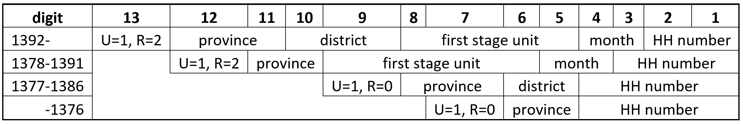
The length and information in variable Address is changing from one year to another. Note that before 1387 the first digit corresponding to rural/urban could be 0/1. If the variable Address is converted to numeric format, before 1387, for rural areas the number of digits in Address is one less. Moreover, note that in years prior to 1382, the Address in the raw data is different from the Address provided in the summary files and the user must build the variable Address based on other variables and the information in the below table. Also in some older years (like 1376) the HH number reported in the data had 5 digits instead of 4. With careful investigation I realized that SCI wrongly inserted a “0” as the second digit of HH number for all household. After removing the second digit I could merge the summary files and raw files.
A minor note on coding: this part of the code can be speeded up using data.table package instead of using summarize of dplyr. But because the dplyr coding is more intuitive I stick to it here. The code using data.table is written in the script in each year.↩︎